Comparing the means of two populations becomes easy with the help of two-sample t-tests. The results of these tests help determine if there is a big difference between the means of the samples.

Furthermore, if the test outcome reports a large difference between the means, it means that the data samples are strong, and the outcome is not because of a sampling error, or worse, random chance.

Two-sample t-tests, also known as Student’s t-tests, can be further classified into two types: paired and unpaired t-tests. Both of these tests have a variety of applications in business, biology, and also psychology.

In this post, we break down what a paired t-test is and when it is appropriate to use the test. We will also dive deep into the hypotheses and assumptions and guide you through doing a test yourself.

What Is A Paired T-Test?

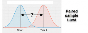
The simplest way to explain paired t-tests is that it is a method that helps determine the mean difference of paired measurements. More specifically, as the hypotheses below reveal, the test helps determine if the difference in the means is zero or not. (musicmundial.com)

The test is known by several other names, including:

Paired samples t-test;
Repeated measures t-test;
Correlated pairs t-test;
Matched-pairs t-test; and
Dependent t-test.

While all its other names explain a lot about the nature of the test, the last name, in particular, can give you more insight into how the test works.

A dependent t-test helps work out if the mean of a dependent variable – which can be anything from patient weight to employee salary – is the same for two related groups.

“Related groups” may be the same group of people being tested, but at different points in time. Think employee salary data before and after training.

The data may also be collected after going through specific conditions.

An excellent example of this is the use of a correlated pairs t-test to determine whether there is a difference in the anxiety levels of a group after using appropriate medication versus taking a placebo.

You cannot use a paired t-test in just any circumstance. You can only use the test if it meets the specific required conditions. Let’s go over those requirements next.

When Can I Use the Test?

You can use the test to:

Find the difference in samples measured at two different points in time.
Determine the difference in data when a group undergoes different conditions.
Work out the difference between two measurements.
Understand the difference between a matched pair.

As long as your goals with hypothesis testing align with any of the four points above, you can use the paired t-test.

Besides that, the data you have at hand must meet the following conditions:

The dependent variable must be continuous – meaning it should either be measured in continuous intervals or ratio levels.
A random sample of data must be selected from the whole population.
The normal distribution must be approximately equal to the difference between the required values.
There shouldn’t be any outliers in the difference between the two groups.
Lastly, the two samples or groups must be related. The subjects in the first sample must also be in the second sample.

We discuss these requirements in more detail in the assumptions section.

When Is Using A Paired T-Test Inappropriate?

If the requirements above are not met, you cannot use a paired t-test. There are also some circumstances where using the paired t-test is inappropriate:

If your data is unpaired, you cannot use the paired samples t-test.
In the event that the data involves comparisons between more than two groups, the test cannot be applied.
The paired t-test cannot be used if the outcome is not normally distributed.
Having an ordinal or ranked outcome dismisses the applicability of the paired t-test.

Hypotheses and Assumptions

Hypotheses

Paired t-tests involve two hypotheses: the null hypothesis (H0) and the alternative hypothesis (H1).

The null hypothesis asserts that there is no difference between the means of the data samples. The hypothesis can be expressed in two mathematically equivalent ways:

H0: µ1 = µ2

And

H0: µ1 – µ2 = 0

On the other hand, the alternative hypothesis asserts a difference between the means of the two data samples. It also declares that the difference is likely not caused by chance or due to a sampling error.

The alternative hypothesis can be expressed in two mathematically equivalent ways:

H1: µ1 ≠ µ2

And

H1: µ1 – µ2 ≠ 0

In the expressions above, µ1 represents the mean of the first group, and µ2 represents the mean of the second group.

Assumptions

Four key assumptions form the basis for a paired t-test, and if even one of these isn’t met, the paired t-test cannot be used to analyze the data.

Even if you try using the test, if the assumptions aren’t met, the result you get will not be valid. Therefore, you must determine whether your study meets the assumptions before performing the paired t-test.

Assumption #1

The dependent variable of the data sample has to be measured at a ratio or interval level. In other words, the variable must be continuous.

Understanding what interval variables and ratio variables mean can be helpful in determining whether your dependent variable is continuous or not.

Interval variables are those variables that you can measure along a continuum. These variables also have a numerical value. Temperature measured in Celsius and Fahrenheit are excellent examples of interval variables.

While ratio variables are also interval variables, a “0” measurement for these variables indicates that there is no variable. A zero measured in Celsius and Fahrenheit doesn’t mean there is no temperature – hence those are not ratio variables. However, if there is a zero measurement in Kelvin, it indicates no temperature, making it a ratio variable.

The height of students, the salary of employees, the scores of a test, and the number of sales per month are some good examples of a dependent variable.

Assumption #2

The independent variable in the data must have two related groups or “matched pairs.” In other words, the two groups should have the same subjects.

To make things a little clearer, the two groups can have the same subjects since the same subjects have been measured on two different occasions (on the same dependent variable).

For instance, you can measure 50 individuals typing speed before and after they completed a typing course. Since the same individuals’ performances were measured at two different instances, the groups of data collected will be related.

Another example of related groups is that two groups of individuals go through two different treatments for the same medical condition to determine which treatment is more effective.

Assumption #3

Besides the independent variable having related groups, there shouldn’t be any significant outliers in the differences between the groups.

Outliers are data points that do not follow the pattern of the data. For instance, if most participants in the typing speed study type at ≈50 WPM, then the individual typing at 100 WPM will be the outlier in the data.

The reasoning behind why the data shouldn’t have significant outliers is that these data points have a negative effect on the t-test. The one really high or really low value can distort the differences between the two groups, reducing the accuracy of the test’s results.

Furthermore, the statistical significance of the test is also affected by the presence of outliers in the data.

Assumption #4

The final assumption the data should meet is that when the distribution of the differences between the groups is plotted out, it should be approximately normally distributed.

Paired t-tests do not require the data to be precisely normal since the assumption can often be violated slightly and still provide valid results.

If you’re unable to discern if the data will violate the normality requirement, you can use the Shapiro-Wilk test to work it out.

It is important to note that ensuring your data meets the third and fourth assumptions will take longer than testing for the first two in practice.

Running the non-parametric Wilcoxon Signed-Ranks Test is a good idea if any of the t-test’s assumptions aren’t met.

How to Perform A Paired T-Test

Assuming that “x” represents the data at a specific time, and “y” represents the data at a later time, you can test the null hypothesis by following these steps:

First, calculate the difference between the two observations for every pair of data (di=yi–xi). It is critical to ensure that you distinguish between the positive and negative values you obtain.
Then, compute the mean difference (d).
Next, calculate the standard deviation of the mean differences (sd).
With the standard deviation handy, find the standard error using the formula SE (d)=sdn.
Now determine the t-statistic using the formula T=dSE (d). Remember that the null hypothesis requires the statistic to have a t-distribution with n-1 degrees of freedom.
To get the p-value, you must use the tables of the t-distribution to get the value of the tn-1 distribution, then compare the t-value to the derived distribution.

Paired T-Test Example

For the sake of understanding how to perform the test, let’s assume that a teacher is trying to work out whether the test she gave this year and the previous year are equally difficult.

The data is as follows:

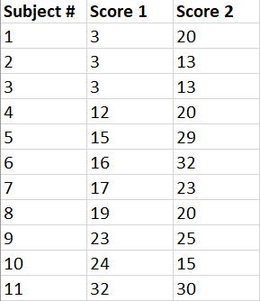
With this data handy, the teacher can measure the mean difference between the scores to determine test difficulty by applying the paired t-test.

The steps the teacher will follow are:

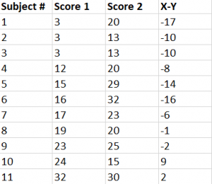
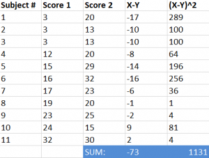
Step #1: Subtract the Y scores from X scores.

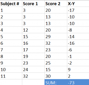
Step #2: Add the values calculated in step #1.

Step #3: Square the values derived in step #1.

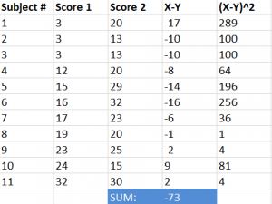
Step #4: Add the values calculated in step #3.

Step #5: Use the formula below to find the t-score

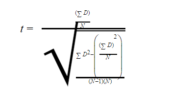
In the formula above,

represents the sum of the differences (from step #2)

represents the sum of the squared differences (from step #4)

represents the sum of the differences (from step #2) squared

Substituting all the values:

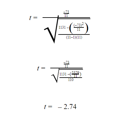
Step #6: Subtract one from the sample to get the required degrees of freedom. Since there are 11 items in the sample, the degrees of freedom are 10.

Step #7: Determine the p-value from the t-table using the determined degrees of freedom. Since there is no alpha-level specified, we will use 0.05 (or 5%).

Since the value of df is 10, the t-value will be 2.228.

Step #8: Compare the value found from the t-table to the calculated value. The calculated value is greater than the table value at the alpha level (we can ignore the polarity of the figure).

Furthermore, the p-value is less than the alpha level (p<0.05). Hence, the teacher can reject the null hypothesis in the test.

Conclusion

Grasping the concept of paired t-tests is quite easy, but applying it requires a focused study of the steps.

Follow the example problem to get a feel for how the test works. Going through the steps a few times will help you get the hang of performing the test faster and interpreting the results correctly.

We have various comprehensive calculators that you can use online for free. You can choose from t-test calculator, graphing, matrix, the standard deviation to statistics, and scientific calculators. Check it here.