A Comprehensive Guide to Limit Comparison Tests

Using the limit comparison test is one of the easier ways to compare the limits of the terms of one series to another and check for convergence. It is different from the direct comparison test and the integral comparison test, both of which are just as well-known.

The direct comparison test compares the terms in the series on an individual basis. On the other hand, the integral test determines the convergence (or divergence) of a series by comparing it to a related improper integral.

The limit comparison test (often shortened to LCT) takes a slightly different approach: comparing the limits on the series of the terms from n to infinity. In other words, the limit comparison test only works for positive values.

While very useful and relatively easy to apply, it can be challenging to understand when to use the convergence test and how to use it effectively.

In this guide, we take you through the heuristics and subtleties of the limit comparison test to help you use it without a struggle.

Limit Comparison Test: The Statement

Let’s assume is an infinite series, where ɑ_n is zero or a positive number. Let’s also assume that there’s a positive sequence b_n that is also positive or zero.

Then:

If is positive and finite, then and either converge or diverge (given that ).
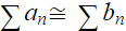If = 0, and converges, then also converges (given that ).
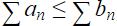If = ∞, and diverges, then also diverges (given that ).

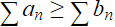Now that you know the statement, it is important to understand the subtleties of cases 2 and 3 above.

Let’s assume that you pick a series to compare with, and you know that the series diverges. Now, if you compute that = 0, you’re essentially arguing that . But since you know that diverges, computing the value doesn’t help you conclude anything.

In the same way, if you pick a series to compare with, and you know that it converges. If you compute that = ∞, you’re essentially arguing that . By the same token, since you know that converges, computing the value doesn’t help you conclude anything.

When to Use LCT

There are three primary scenarios you can apply the limit comparison test in. There’s a fourth, broad scenario where the LCT can be helpful too.

Case 1: Isolating Dominant Terms

The LCT is the most useful and most straightforward method to isolate the dominant behavior in a series. If a series has dominant terms that are apparent when you first look at the series, it is possible to generate a bn to compare the series with, by isolating the series’ dominant behavior.

Here’s an example to explain this:

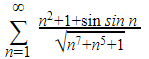
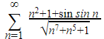
At first glance, there’s a lot you can ignore in the series. There are three terms in the numerator. The first term, n², is the most important term because n grows to infinity in this series. The second term, 1, cannot grow. And finally, the third term sin n bounces between the interval of -1 and 1 depending on the value of n.

Since sin n is very different from sin (1/n), we are not in case 3 mentioned in the statement of LCT.

Now, looking at the denominator, you will find three terms under the square root. Since there is a √n⁷, the dominant behavior in the denominator comes from √n⁷.

Knowing all of this, intuitively, we can work this expression down:

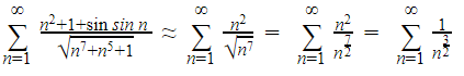
Now, the resulting p-series is convergent, and therefore, we can intuitively say that is also convergent.

We can formalize this idea using the limit comparison test:

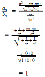
One is finite and positive, meeting the criteria of case 1. This means that the series

And the series

Both converge or diverge. Since the latter series is convergent, we can conclude that the former series is also convergent.

Case 2: Logarithms

When there are logarithms in a series, they introduce some subtleties and challenges in limit comparison.

What you need to remember is this:

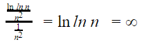
ln ln n “n^a (given that a > 0)

And also:

(ln ln n )<^p “n^a (given that a > 0 and p > 0)

You can infer from these notes that the growth of a logarithm in a series can be absorbed with a small power of n.

More specifically, you can infer that if a series has a logarithm that cannot be ignored, you can create a series to compare it with by replacing ln ln n with a small power of n.

When you do this, the logarithmic growth in the series is gone. The LCT will likely be in case 2 or case 3 of the statement.

Here’s an example to explain this:

In this example, the denominator grows at the rate of n². But what’s more interesting is that the numerator grows slower than n².

We can formalize this idea by running LCT. But we can’t simply ignore the logarithm in the series and replace it with one. Here’s what happens if we ignore the logarithm:

If you look at the criteria of case 3 in the statement, we can only make a conclusion if the series in the denominator diverges. But , and and doesn’t reveal that the series is divergent.

So, testing by ignoring the logarithm is inconclusive. And this should be taken as a warning that while the growth of the logarithm is slow, it cannot be ignored.

We will need to consider a small amount of growth to absorb the logarithm. So, we can use the heuristic:

ln ln n ⇝n^{small #}

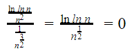
If we use the heuristic instead of ln ln n in the expression, we get:

Since we want to prove that the series is convergent, we must first show that the series is convergent.

To prove this, n^{2-(small #)} must be greater than one.

If n^{2-(small #)}> 1, then 0 < small # < 1. Let’s assume that small # = ½ and run the LCT.

Now that we’ve gotten a limit of zero from the test, and know for a fact that converges, we can apply case 2 from the statement and conclude that also converges.

Case 3: Trigonometric Functions and Taylor Polynomials

Let’s consider the graph of a regular sine function.

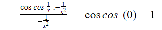
When you plot the y = sin(x) graph, you will find that the tangent line at x=0 is y=x. The reasoning behind this is simple: sin(0) is equal to zero, and cos(0) is equal to one.

Using the Meta-Calculator graphing calculator, we’ve plotted the intersection of both equations on the graph.

The graph makes it clear that sin(x) is approximately equal to x when x is close to 0. Additionally, the fraction has a value close to 0 for large values of n.

This proves that sin sin . We can exploit this property of the sine function to create useful comparison candidates for the LCT.

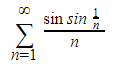
Consider this example series:

Considering the proof above, we can intuitively find that:

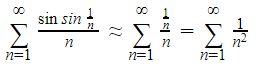
We can formalize this idea by using the LCT.

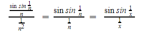
Applying L’Hospital rule:

Now, since one is a positive and finite number, we find ourselves in case 1 of the LCT statement. In other words, the series and have the same behavior. Since the latter converges, according to the statement, we can be sure that the former also converges.

Many other approximations can prove useful in generating series for comparison. Some of them include:

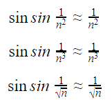
There are many ways to manipulate these approximations to generate more approximations. You can read about them here.

What you must bear in mind is that sin sin x ≈ x only when x is small. For the approximations to hold, the value in the sine function must tend to 0. For this reason, we cannot make assumptions like sin sin n ≈ n.

Taylor Polynomial Approximations

Applying the knowledge we have of Taylor polynomials generally allows us to capture the behavior of other sequences.

For instance, the degree 2 Taylor polynomial for cos(x) at 0 is:

In other words, when x is near 0, we can approximate:

We can use this approximation just we used the approximation in the case of sin(x). For instance, consider the following series:

The general behavior can be identified as:

After arriving at this result, we can use the LCT to verify that has the same behavior that does, and therefore, the series converges.

But this is only one example of using Taylor polynomials generating approximations. There are many others that you can use. For instance, a degree 1 Taylor polynomial for e^x at 0 is:

In other words, we can expect e^x≈1 + x when x is near 0. With this approximation, we can make sequential approximations such as:

Case 4: Catch-All Case

There are scenarios that you cannot identify with any of the above cases. In such scenarios, you can choose to run an LCT against .

It’s important to note that this doesn’t always work. But a lot of times, it can give you the answer.

There are two scenarios where you can apply this method and be sure that it’ll work:

If you believe is a diverging series, run an LCT against .
If you believe is a converging series, run an LCT against .

The reason why this works for a lot of series is that is the biggest infinite series that is convergent. In other words, it converges, but very slowly.

On the other hand, is among the smallest divergent series – it diverges, but very slowly.

Proving convergence via comparison requires you to compare a series with another series that is bigger and also converges. By the same token, if you want to prove divergence by comparing, you will need to compare the series with a smaller series that also diverges. (wealthymint)

Heuristically, the series is bigger than the majority of other convergent series, which makes it a good candidate for convergent comparison. Likewise, is a good candidate for divergent comparison.

Meta-Calculator Limit Calculator

You don’t always need to have a scientific calculator at hand to calculate limits. You can use the Meta-Calculator limit calculator to work out the limits of functions.

It is accessible from any device with an internet connection. Further, it is completely free to use, making it one of the handiest limit calculators you’ll come across.

Besides being easy to use and passing you results instantly, it supports finding a limit as x with any number – including infinity.

Meta-Calculator also offers a graphing tool, as you may have seen in the case 3 section earlier. Getting a visual understanding of a function is as simple as entering the function in the tool. You can also enter two functions and have Meta-Calculator draw an intersection between the graphs.

To find the limit of any function using the Meta-Calculator Limit Calculator:

Navigate to the Meta-Calculator Limit Calculator from a browser of your choice. The calculator looks like this:
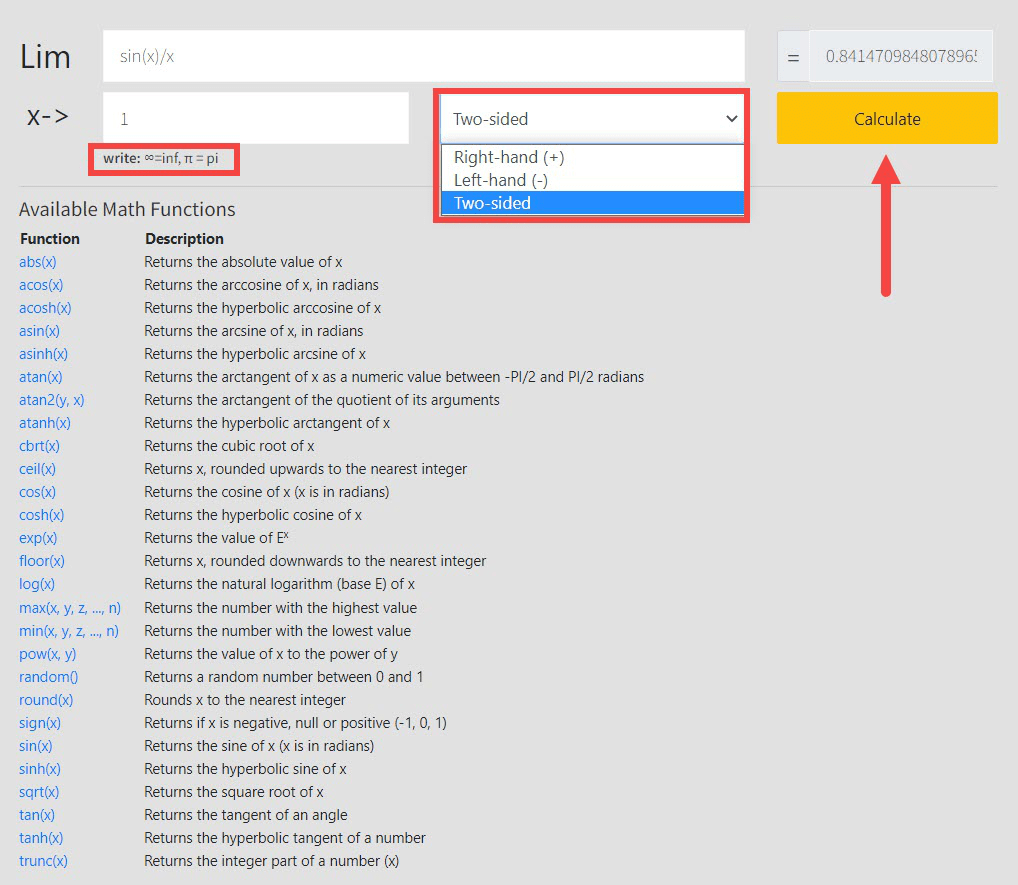
Type in the function that you want to calculate the limit of in the input box.
Enter the arrow number in the designated box.
Choose whether you want a two-sided calculation, or just from the right or the left hand.
Click “Calculate.” Meta-Calculator will calculate the limit of the function.
To calculate the limit of another function, clear the input boxes and repeat from step 2.

In addition to trigonometric functions, you can work with hyperbolic functions, arc functions, logarithms, and square roots. Meta-Calculator offers several functions to work out limits on the go or at your computer, as long as you’re connected to the internet.

Functions such as abs(x) and floor(x) are also available. With these, you can feed any function you need to find the limit on Meta-Calculator easily.